


Slope Fields with Mathematica - Exercise 3.3
Making Slope Fields by Yourself
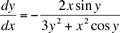
A Post Exercise Discussion of
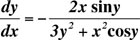
on the region -3 ≤ x ≤ 3, and -3 ≤ y ≤ 3
Don't cheat! If you didn't do the exercise in Mathematica before you came here to see the discussion, go back and do it now!
Assuming that you did the exercise correctly, you should have produced a picture that was a version of the following:

As you can see, once again neither horizontal nor vertical lines are isoclines. Finding the isoclines analytically, (the same way we did in the last two exercises), leads to:
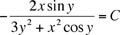 .
.where C represents any constant.
I personally don't have a clue what the graph of this equation looks like. To get much insight from the isocline equation would require having Mathematica help us with the graphing difficulties. This time the required work is much more complicated, since the isoclines found above are defined implicitly, and to make Mathematica plot implicitly defined curves requires the loading of yet another external package. Furthermore, the isocline curve families don't plot well, as they fall into distinct sub-families for each quadrant of the plane. To get decent looking images, it helps to have Mathematica do a separate plot for each quadrant, and then combine these together for the final image. Once all of this hard work is over, the resulting graph looks something like this:
Try to verify from this image that as you trace along any particular one of the red isoclines, the slopes of the vectors which intersect it are all the same.
| You will not be asked to graph isoclines like this on lab exams, but if you'd like to see the Mathematica notebook that was used to make the above plot, click on the icon to the left. If you do, please try to read it carefully, and try to understand what each command is being used for. Feel free to experiment with it a little. Don't forget to return here when you are done. |
What about finding an analytic solution? This problem is of a class of differential equations referred to as exact. You may or may not have learned how to solve exact differential equations analytically already in the lecture part of your course. Unfortunately, unlike separation of variables, which we covered in the previous problem, this method relies on a little more than just simple algebra and simple calculus for solution. Once you learn the right technique you'll see that exact differential equations aren't too hard to solve.
Using this technique, it can be shown that the actual analytic solution to this problem, in implicit form, is:
Sadly we have a hard time visualizing this one too. As before, we let Mathematica do the heavy lifting. Doing so we arrive at the following image:
As you can see, the solution curves that we just calculated theoretically fit the slope field that we made earlier quite well.
| You will not be asked to graph solutions curves over slope fields like this on lab exams, but if you'd like to see the Mathematica notebook that was used to make the above plot, click on the icon to the left. If you do, please try to read it carefully, and try to understand what each command is being used for. Feel free to experiment with it a little. Don't forget to return here when you are done. |
We're now done with the discussion of this problem, so let's go back to the exercises.
 |
If you're lost, impatient, want an overview of this laboratory assignment, or maybe even all three, you can click on the compass button on the left to go to the table of contents for this laboratory assignment. |