Slope Fields with Mathematica - Exercise 3.2

Don't cheat! If you didn't do the exercise in Mathematica before you came here to see the discussion, go back and do it now!

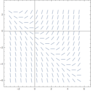
Assuming that you did the exercise correctly, you should have produced a picture that was simply a larger version of the following:

This time it is quite obvious that neither horizontal nor vertical lines are isoclines for this slope field. It looks like finding the isoclines will be more of an analytical rather than a visual procedure.

Just as in the previous exercise, we can find the isoclines by looking for curves along which the slope, (the derivative), is constant.

The differential equation tells us:

which we can think of as:

But isoclines are where slope is constant. So let's rewrite the equation again as:

Or, more briefly as:

where C represents any constant. A little algebra, (very little), gives us:

Now, since the equation y = -x + C describes the shape of the isoclines of this slope field we can see that we are back to having straight line isoclines in this problem. The difference from our past experience is that the lines are slanted. Indeed, apparently they all have a slope of -1.

Looking back at the slope field picture again, can you see that if you move along any line of slope -1, the field marks all have identical slopes? If you can't see this then feel free to return to Mathematica and redraw the slope field using a higher density of shorter field marks as we've done a couple of times already in other exercises.

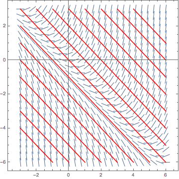
Or if you took the time to read my example notebook on using Mathematica to draw the isoclines over the slope field in the previous example, you might feel ambitious enough to try using it yourself now to do the same with this new problem! If you do, the results end up looking something like this:

Try to verify from this image that as you trace along any particular one of the red linear isoclines, the slopes of the vectors which intersect it are all the same.

You will not be asked to graph isoclines like this on lab exams, but if you'd like to see the Mathematica notebook that was used to make the above plot, click on the icon to the left. If you do, please try to read it carefully, and try to understand what each command is being used for. Feel free to experiment with it a little. Don't forget to return here when you are done.

Now, what about finding an analytic solution? This problem is of a class of differential equations referred to as linear . You may or may not have learned how to solve linear differential equations analytically already in the lecture part of your course. Unfortunately, unlike separation of variables, which we covered in the previous problem, this method relies on a little more than just simple algebra and simple calculus for solution. Once you learn the right technique you'll see that linear differential equations are really quite easy to solve.

Using this technique, it can be shown that the actual analytic solution to this problem is:

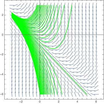
At least this time we stand a chance of recognizing what the pictures of the members of this family of curves look like. This solution is actually just the sum of three functions which are quite familiar to us, namely C e^x , -x, and -1. Remembering that the C merely acts to change the "slope" of the exponential growth function, it's not too hard to see that these solutions really do match the trend of the slope field. In fact, once again, we could use Mathematica to superimpose its graph on the slope field and compare. If we do this, the result would look something like the following:

As you can see, the solution curves that we just calculated theoretically fit the slope field that we made earlier quite well.

You will not be asked to graph solutions curves over slope fields like this on lab exams, but if you'd like to see the Mathematica notebook that was used to make the above plot, click on the icon to the left. If you do, please try to read it carefully, and try to understand what each command is being used for. Feel free to experiment with it a little. Don't forget to return here when you are done.

We're done with the discussion of this problem, so let's go back to the exercises.