Slope Fields with Mathematica

(continued from last page...)

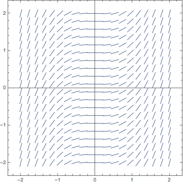
Your trip to Mathematica should have given a result like this:

Our preliminary example as drawn by Mathematica,
now with a 20 X 20 grid of vectors, all of equal length.

Notice how we now have a much finer array of vectors, and a better feel for how the true solutions to the original differential equation might snake their way across the Cartesian plane.

Now for a little analysis of the above slope field...

Do you notice how the slopes in the slope field you just formed only depend upon x, but not on y? i.e. if you move up or down any vertical line in the plane, all of the slopes along it are identical. Why is this? Well, it has to do with our differential equation. Remember, the slope at any point was given by:

So there wasn't any y in the formula for slope, just x. This dependence of the slope (or the derivative, if you prefer) upon a single variable will not always be the case. As is usual in mathematics, we made the first example an extra easy one!

Now any curve on a slope field diagram along which all of the slope field's slopes are the same is referred to as an isocline. According to this definition, then, for the example we just did with Mathematica any vertical line through the slope field would be an isocline. It should be noted that, in general, isoclines need not be straight lines.

We'll come back and do a little more theory shortly, but now it's time to look at whether you can make Mathematica plot a slope field without me telling you exactly what to type.