Slope Fields with Mathematica - Exercise 3.4

Don't cheat! If you didn't do the exercise in Mathematica before you came here to see the discussion, go back and do it now!

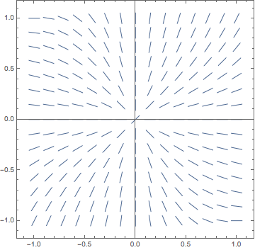
Assuming that you did the exercise correctly, you should have produced a picture like this:

It should be clear that there is some kind of origin symmetry evident in the slope field.

Moving more quickly, since we've had so much experience by now, we know the equation of the isocline family is:

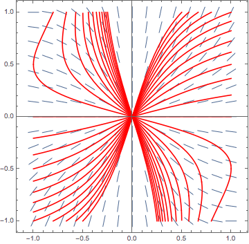
which is kind of unrecognizable. It is possible to solve this for y using the quadratic formula, and then make a graph, but that looks like more trouble than it's worth, especially if Mathematica can be pressed into service for the task. Doing this, we produce a plot looking much like the following:

Try to verify from this image that as you trace along any particular one of the red isoclines, the slopes of the vectors which intersect it are all the same.

You will not be asked to graph isoclines like this on lab exams, but if you'd like to see the Mathematica notebook that was used to make the above plot, click on the icon to the left. If you do, please try to read it carefully, and try to understand what each command is being used for. Feel free to experiment with it a little. Don't forget to return here when you are done.

What about finding an analytic solution? This problem is of a class of differential equations referred to as Bernoulli equations, (named after Swiss mathematician Jakob Bernoulli.) You may or may not have learned how to solve Bernoulli equations analytically in the lecture part of your course yet.

Using Bernoulli's technique, it can be shown that the actual analytic solution to this problem is:

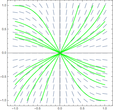
Again, Mathematica can be talked into helping with the plot, producing:

As you can see, the solution curves that we just calculated theoretically fit the slope field that we made earlier quite well.

You will not be asked to graph solutions curves over slope fields like this on lab exams, but if you'd like to see the Mathematica notebook that was used to make the above plot, click on the icon to the left. If you do, please try to read it carefully, and try to understand what each command is being used for. Feel free to experiment with it a little. Don't forget to return here when you are done.

We're done with the discussion of this problem, so let's go back to the exercises.