Slope Fields with Mathematica - Exercise 3.1

Don't cheat! If you didn't do the exercise in Mathematica before you came here to see the discussion, go back and do it now!

Assuming that you did the exercise correctly, you should have produced a picture that looked somewhat like the following:

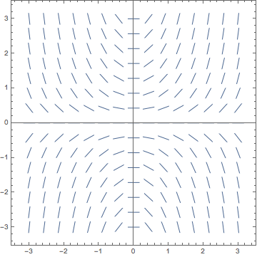
At first glance it may seem that the field marks once again have matching slopes along vertical lines, but look more closely. This impression is simply a result of the graph's y-axis symmetry. In actual fact it looks like the slopes of the field marks get steeper the further away you go from the x-axis. For the first time in this laboratory we are witnessing a slope field whose isoclines are neither vertical nor horizontal. In fact the isoclines of this field are not even straight lines!

So what are they? Well, let's remind ourselves of the definition of the word isocline—a curve in the slope field along which all of the field marks have the same slope. i.e. to find an isocline, (especially if you can't find it easily just by looking at the graph as we've done in the past), look for where the slope is constant.

So let's reason as follows:

The differential equation tells us:

which we can think of as:

But we said a little earlier that isoclines are where slope is constant. So let's rewrite the equation again as:

Or, more briefly as:

where C represents any constant.

So the equation x y = C describes the shape of the isoclines of this slope field. Do you recognize it? It may take a little digging in the deep recesses of your memory to come up with the fact that this curve is a hyperbola for any non-zero value of C. (Actually, it's a hyperbola rotated 45 degrees from it's standard position.)

Now that you know that the isoclines are hyperbolas, can you see them? Well, don't feel bad, neither can I. To be able to pick out the isoclines clearly we would need to redo the problem with a much denser slope field, and then superimpose some sample curves from the family x y = C on the field itself. Tracing our way along any of these superimposed curves we should find that all of the field marks intersecting the isocline have exactly the same slopes. It is actually possible to achieve this effect with Mathematica, and the results end up looking something like this:

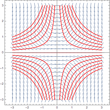
It's still a little tough to see clearly, but try to verify from this image that as you trace along any particular one of the red hyperbolic isoclines, the slopes of the vectors which intersect it are all the same.

You will not be asked to graph isoclines like this on lab exams, but if you'd like to see the Mathematica notebook that was used to make the above plot, click on the icon to the left. If you do, please try to read it carefully, and try to understand what each command is being used for. Feel free to experiment with it a little. Don't forget to return here when you are done.

Make sure you understand the theoretical procedure we used to find the isoclines above—the same method works on all first order differential equations that can be written in the form dy/dx = g(x, y).

Anyway, enough about isoclines, what about finding an analytic solution? This problem can be solved by a method similar to the one we've used so far, i.e. direct integration. The method is referred to as separation of variables. The general idea being that we rewrite the differential equation in the form:

Now this change is not always possible for every equation. The one's which can be rearranged this way are called separable.

Here goes! Starting with:

we multiply both sides by dx, and divide both sides by y to get:

Now from here integration is simple. We get:

A little algebraic rearranging to isolate y gives us:

Whether or not the slope field we see looks anything like the family of curves we have just written is a little elusive since most of us never memorized the graph of e^x2/2. However, we could use Mathematica to superimpose its graph on the slope field and compare. If we do this, the result would look something like the following:

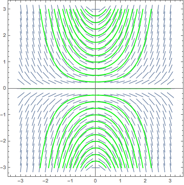
As you can see, the solution curves that we just calculated theoretically fit the slope field that we made earlier quite well.

You will not be asked to graph solutions curves over slope fields like this on lab exams, but if you'd like to see the Mathematica notebook that was used to make the above plot, click on the icon to the left. If you do, please try to read it carefully, and try to understand what each command is being used for. Feel free to experiment with it a little. Don't forget to return here when you are done.

Well, we're done with the discussion of this problem, so let's go back to the exercises.