Slope Fields with Mathematica - Exercise 2.4
Making Slope Fields by Yourself
A Post Exercise Discussion of
dy/dx = ey, on the region -1 ≤ x ≤ 1, and -1 ≤ y ≤ 1
Don't cheat! If you didn't work the exercise in Mathematica before you came here to see the discussion, go back and do it now!
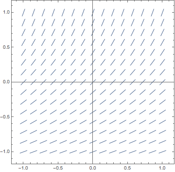
Assuming that you worked the problem correctly, you should have produced a picture similar to this:

The horizontal isoclines are evident once again in this picture. Obviously we're seeing a common theme running through all slope fields of equations of this general type.
But do we recognize the slope field trend? Let's go for the analytic solution right away and see if we can spot a connection.
Starting with:
We first divide both sides by ey, to get:
Which can be rewritten as:
Now we integrate both sides individually to get:
A little basic algebra allows us to isolate the y here to give:
This describes a family of upside down natural logarithm functions each shifted horizontally from the others by the movement resulting from changing the value of C. The picture does seem to agree with this analysis. If you don't quite see the agreement yourself, try returning to Mathematica and experimenting further with the bounds of the plot, and maybe even the number of vectors being plotted.
Well, we're done with the discussion of this problem, so let's go back to the exercises.


