Numerical Methods - Euler Method Summary

Numerical Methods for Solving Differential Equations

Euler's Method

Theoretical Introduction

(continued from last page...)

Summary of Euler's Method

In order to use Euler's Method to generate a numerical solution to an initial value problem of the form:

y′ = f(x, y)

y(x_o) = y_o

we decide upon what interval, starting at the initial condition, we desire to find the solution. We chop this interval into small subdivisions of length h. Then, using the initial condition as our starting point, we generate the rest of the solution by using the iterative formulas:

x_n+1 = x_n + h

y_n+1 = y_n + h f(x_n, y_n)

to find the coordinates of the points in our numerical solution. We terminate this process when we have reached the right end of the desired interval.

A Preliminary Example

Just to get a feel for the method in action, let's work a preliminary example completely by hand. Say you were asked to solve the initial value problem:

y′ = x + 2y

y(0) = 0

numerically, finding a value for the solution at x = 1, and using steps of size h = 0.25.

Applying the Method

Clearly, the description of the problem implies that the interval we'll be finding a solution on is [0,1]. The differential equation given tells us the formula for f(x, y) required by the Euler Method, namely:

f(x, y) = x + 2y

and the initial condition tells us the values of the coordinates of our starting point:

• x_o = 0
• y_o = 0

---

We now use the Euler method formulas to generate values for x₁ and y₁.

The x-iteration formula, with n = 0 gives us:

x₁ = x_o + h

or:

x₁ = 0 + 0.25

So:

x₁ = 0.25

And the y-iteration formula, with n = 0 gives us:

y₁ = y_o + h f(x_o, y_o)

or:

y₁ = y_o + h (x_o + 2y_o)

or:

y₁ = 0 + 0.25 (0 + 2*0)

So:

y₁ = 0

Summarizing, the second point in our numerical solution is:

• x₁ = 0.25
• y₁ = 0

---

We now move on to get the next point in the solution, (x₂, y₂).

The x-iteration formula, with n=1 gives us:

x₂ = x₁ + h

or:

x₂ = 0.25 + 0.25

So:

x₂ = 0.5

And the y-iteration formula, with n = 1 gives us:

y₂ = y₁ + h f(x₁, y₁)

or:

y₂ = y₁ + h (x₁ + 2y₁)

or:

y₂ = 0 + 0.25 (0.25 + 2*0)

So:

y₂ = 0.0625

Summarizing, the third point in our numerical solution is:

• x₂ = 0.5
• y₂ = 0.0625

---

We now move on to get the fourth point in the solution, (x₃, y₃).

The x-iteration formula, with n = 2 gives us:

x₃ = x₂ + h

or:

x₃ = 0.5 + 0.25

So:

x₃ = 0.75

And the y-iteration formula, with n = 2 gives us:

y₃ = y₂ + h f(x₂, y₂)

or:

y₃ = y₂ + h (x₂ + 2y₂)

or:

y₃ = 0.0625 + 0.25 (0.5 + 2*0.0625)

So:

y₃ = 0.21875

Summarizing, the fourth point in our numerical solution is:

• x₃ = 0.75
• y₃ = 0.21875

---

We now move on to get the fifth point in the solution, (x₄, y₄).

The x-iteration formula, with n = 3 gives us:

x₄ = x₃ + h

or:

x₄ = 0.75 + 0.25

So:

x₄ = 1

And the y-iteration formula, with n = 3 gives us:

y₄ = y₃ + h f(x₃, y₃)

or:

y₄ = y₃ + h (x₃ + 2y₃)

or:

y₄ = 0.21875 + 0.25 (0.75 + 2*0.21875)

So:

y₄ = 0.515625

Summarizing, the fourth point in our numerical solution is:

• x₄ = 1
• y₄ = 0.515625

---

We could summarize the results of all of our calculations in a tabular form, as follows:

n	xn	yn
0	0.00	0.000000
1	0.25	0.000000
2	0.50	0.062500
3	0.75	0.218750
4	1.00	0.515625

A question you should always ask yourself at this point of using a numerical method to solve a problem, is "How accurate is my solution?" Sadly, the answer is "Not very!" This problem can actually be solved without resorting to numerical methods (it's linear). The true solution turns out to be:

y = 0.25 e^2x - 0.5 x - 0.25

If we use this formula to generate a table similar to the one above, we can see just how poorly our numerical solution did:

x	y
0.00	0.000000
0.25	0.037180
0.50	0.179570
0.75	0.495422
1.00	1.097264

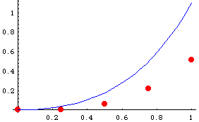
We can get an even better feel for the inaccuracy we have incurred if we compare the graphs of the numerical and true solutions, as shown here:

The numerical solution gets worse and worse as we move further to the right. We might even be prompted to ask the question "What good is a solution that is this bad?" The answer is "Very little good at all!" So should we quit using this method? No! The reason our numerical solution is so inaccurate is because our step-size is so large. To improve the solution, shrink the step-size!

By the way, the reason I used such a large step size when we went through this problem is because we were working it by hand. When we move on to using the computer to do the work, we needn't be so afraid of using tiny step-sizes.

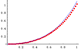
To illustrate that Euler's Method isn't always this terribly bad, look at the following picture, made for exactly the same problem, only using a step size of h = 0.02:

As you can see, the accuracy of this numerical solution is much higher than before, but so is the amount of work needed! Look at all those red points! Can you imagine calculating the coordinates of each of them by hand?

I think that we have adequately demonstrated the concepts underlying the Euler's Method algorithm. We have seen the derivation of the required formulas from both a graphical and a formulaic point-of-view. We've even gone through an example of using the method for a small number of points. Now it's time to get out the big guns! This method is one that truly belongs on a computer!

Let's now go and see how we would implement these ideas in Mathematica.

---

If you're lost, impatient, want an overview of this laboratory assignment, or maybe even all three, you can click on the compass button on the left to go to the table of contents for this laboratory assignment.