Numerical Methods - Euler Method Part 2

Numerical Methods for Solving Differential Equations

Euler's Method

Theoretical Introduction

(continued from last page...)

Developing Euler's Method Graphically

In order to develop a technique for solving first order initial value problems numerically, we should first agree upon some notation. We will assume that the problem in question can be algebraically manipulated into the form:

y′ = f(x, y)

y(x_o) = y_o

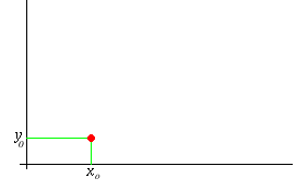
Our goal is to find a numerical solution, i.e. we must find a set of points which lie along the initial value problem's solution. If we look at this problem, as stated above, we should realize that we actually already know one point on the solution, namely the one defined by the initial condition, (x_o, y_o). Possibly, the picture of this tiny piece of information looks something like this:

Now, remember we don't really know the true solution of the problem, or we wouldn't be going through this method at all. But let's act as if we do know this elusive solution for a moment. Let's pretend that it's "ghostly graph" could be superimposed onto our previous picture to get this:

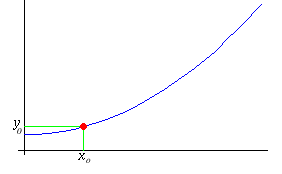
Again, the blue graph of the true solution, shown above, is actually unknown. We've drawn a picture of what it might look like just to help us think.

Since we're after a set of points which lie along the true solution, as stated above, we must now derive a way of generating more solution points in addition to the solitary initial condition point shown in red in the picture. How could we get more points?

Well, look back at the original initial value problem at the top of the page! So far we have only used the initial condition, which gave us our single point. Maybe we should consider the possibility of utilizing the other part of the initial value problem—the differential equation itself:

y′ = f(x, y)

Remember that one interpretation of the quantity y′ appearing in this expression is as the slope of the tangent line to the function y. But, the function y is exactly what we are seeking as a solution to the problem. This means that we not only know a point which lies on our elusive solution, but we also know a formula for its slope:

slope of the solution = f(x, y)

All we have to do now is think of a way of using this slope to get those "other points" that we've been after! Well, look at the right hand side of the last formula. It looks like you can get the slope by substituting values for x and y into the function f. These values should, of course, be the coordinates of a point lying on the solution's graph—they can't just be the coordinates of any point anywhere in the plane. Do we know of any such points—points lying on the solution curve? Of course we do! The initial condition point that we already sketched is exactly such a point! We could use it to find the slope of the solution at the initial condition. We would get:

slope of the solution at (x_o, y_o) = f(x_o, y_o)

Remembering that this gives us the slope of the function's tangent line at the initial point we could put this together with the initial point itself to build the tangent line at the initial point, like this:

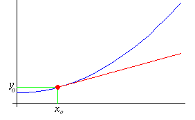
Once again, let's remind ourselves of our goal of finding more points which lie on the true solution's curve. Using what we know about the initial condition, we've built a tangent line at the initial condition's point. Look again at the picture of this line in comparison with the graph of the true solution in the picture above. If we're wanting other points along the path of the true solution, and yet we don't actually have the true solution, then it looks like using the tangent line as an approximation might be our best bet! After all, at least on this picture, it looks like the line stays pretty close to the curve if you don't move too far away from the initial point.

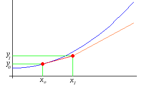
Let's say we move a short distance away, to a new x-coordinate of x₁. Then we could locate the corresponding point lying on our tangent line. (We can't do this for the curve—it's a ghost, remember!) It might look something like this:

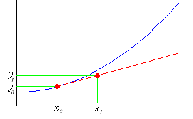
Notice that our new point, which I've called (x₁, y₁), isn't too terribly far away from the true value of the solution at this x-coordinate, up on the curve.

So we now have two points as part of our numerical solution:

• (x_o, y_o): an exact value, known to lie on the solution curve.
• (x₁, y₁): an approximate value, known to lie on the solution curve's tangent line through (x_o, y_o).

We must now attempt to continue our quest for points on the solution curve (though we're starting to see the word "on" as a little optimistic—perhaps "near" would be a more realistic word here.) Still glowing from our former success, we'll dive right in and repeat our last trick, constructing a tangent line at our new point, like this:

You should immediately recognize that there's a problem, and I've cheated to overcome it! Since our new point didn't actually lie on the true solution, we can't actually produce a tangent line to the solution at this point. (We don't even know where the true solution actually is anymore—the blue curve in the picture is just a thinking aid.) But we can still substitute our new point, (x₁,y₁), into the formula:

slope of the solution = f(x,y)

to get get the slope of a pseudo-tangent line to the curve at (x₁,y₁). We hope that our approximate point, (x₁,y₁), is close enough to the real solution that the pseudo-tangent line is pretty close to the unknown real tangent line.

We now attempt to use this new pseudo-tangent line to get yet another point in the approximate solution. As before, we move a short distance away from our last point, to a new x-coordinate of x₂. Then we locate the corresponding point lying on our pseudo-tangent line. The result might look something like this:

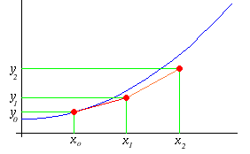
We now have three points in our approximate solution:

• (x_o, y_o): an exact value, known to lie on the solution curve.
• (x₁, y₁): an approximate value, known to lie on the solution curve's tangent line through (x_o, y_o).
• (x₂, y₂): an approximate value, known to lie on the solution curve's pseudo-tangent line through (x₁, y₁).

As you can see, we're beginning to establish a pattern in the way we are generating new points. We could continue making new points like this for as long as we liked, but for the sake of this illustration let's find just one more value in the approximate solution.

We make another pseudo-tangent line, this time through (x₂, y₂), like this:

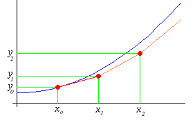
and we make another short jump to an x-coordinate of x₃, and locate the corresponding point on our latest pseudo-tangent line, like this:

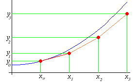
So the list of points in our approximate numerical solution now has four members:

• (x_o, y_o): an exact value, known to lie on the solution curve.
• (x₁, y₁): an approximate value, known to lie on the solution curve's tangent line through (x_o, y_o).
• (x₂, y₂): an approximate value, known to lie on the solution curve's pseudo-tangent line through (x₁, y₁).
• (x₃, y₃): an approximate value, known to lie on the solution curve's pseudo-tangent line through (x₂, y₂).

Looking over the picture one last time, we see an example of how the numerical solution—the red dots, might compare with the actual solution. As we stated in the introduction to this laboratory, a weakness of numerical solutions is their tendency to drift away from the true solution as the points get further away from the initial condition point. One way of minimizing (but not eliminating) this problem is to make sure that the jump-size between consecutive points is relatively small.

Now that you've seen the pictorial version of Euler's Method for finding numerical solutions, you should have a better chance of understanding the derivation of the formulas used by the method. So, let's go and derive them...

If you're lost, impatient, want an overview of this laboratory assignment, or maybe even all three, you can click on the compass button on the left to go to the table of contents for this laboratory assignment.