Solving the Preliminary Example

continued from last page...)

Your fairly lengthy session should have gone something like this:

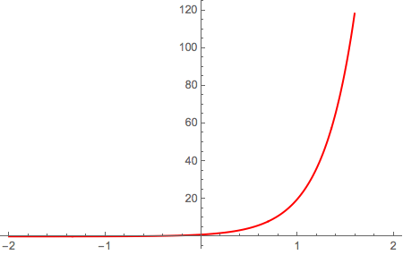
prelimyplot= Plot[prelimy,{t,-2,2},
  PlotStyle->RGBColor[1,0,0]]



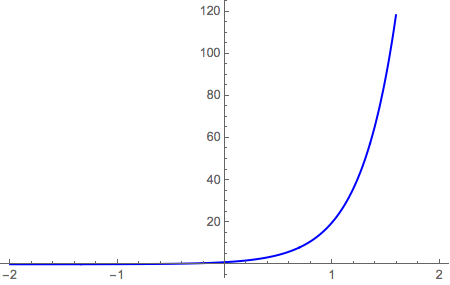
proposedyplot= Plot[E^(3t), {t,-2,2},
  PlotStyle->RGBColor[0,0,1]]



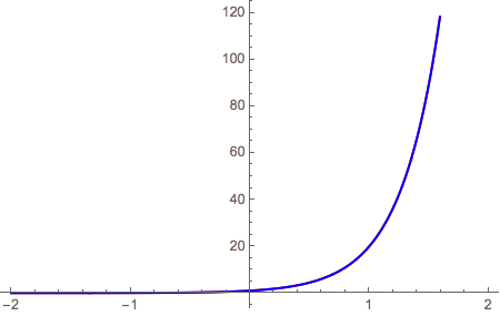
Show[prelimyplot,proposedyplot]

Once again we can see that the two graphs are indistinguishable in the final plot. It appears that, at least based on this one example, the numerical solver routines built into Mathematica are quite reliable when applied to systems of differential equations. In most problems we will not have the luxury of knowing the solution ahead of time, as we did here, so we won't be able to compare the numerical solution to anything else. This is why we've taken the time to go through this preliminary example carefully so that we can build a little confidence in our solver.

We now move on so that you can do a few exercises solo...

If you're lost, impatient, want an overview of this laboratory assignment, or maybe even all three, you can click on the compass button on the left to go to the table of contents for this laboratory assignment.