Slope Fields with Mathematica - Exercise 2.3
Making Slope Fields by Yourself
A Post Exercise Discussion of
dy/dx = cos y, on the region -5 ≤ x ≤ 5, and π ≤ y ≤ π
Don't cheat! If you didn't do the exercise in Mathematica before you came here to see the discussion, go back and do it now!
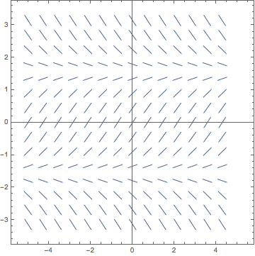
Assuming that you did the exercise correctly, you should have produced a picture that was simply a larger version of the following:

Yet another one with horizontal isoclines.
The slope field has such a complicated flow to it that it's almost impossible to spot any kind of trend. This calls for further investigation!
Up until now, I've been telling you the setting I would recommend for the VectorPoints option of the VectorPlot command. As you can see from the above results, sometimes it will be necessary for you to make a decision for yourself as to whether this option requires adjustment in order to get a better feel for the true nature of a slope field.
Reworking the Exercise
Just as a reminder, the original problem was to make the slope field of:
What I'd like you to do is go to Mathematica (in just a second—hold on) and make the following changes to the way you did the problem before:
- Change the plot bounds to: -5 ≤ x ≤ 5, and -2π ≤ y ≤ 2π. This will provide us a larger overview of the plot field.
- Increase the VectorPoints value to a higher value, (experiment a little if necessary)
Now go back to Mathematica and make these changes, coming back here when you are done.
Welcome back! Did you get a slightly better feel for the slope field now that you redid the exercise with the suggested changes? Obviously we now need to further discuss our latest discoveries.


