Slope Fields with Mathematica - Exercise 1.1
Making Slope Fields by Yourself
A Post Exercise Discussion of
dy/dx = x, on the region -3 ≤ x ≤ 3, and -3 ≤ y ≤ 3
I hope you actually did do the exercise in Mathematica before you came here to see the discussion. Your purpose is to learn how to do these things for yourself, after all, not to read the computer screen as if it were just a book. If you didn't do it yet, go back and do the exercise now!
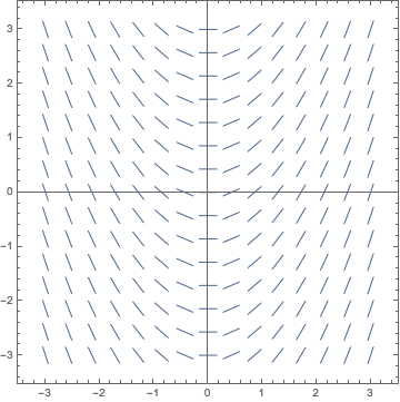
Anyway, assuming that you did the exercise correctly, you should have produced a picture very much like the following:

You should have already noticed that the isoclines for this slope field are once again vertical lines, (just like in our preliminary example.) Do you recognize the general trend of the field? Kind of parabolic, right? Does this make sense if you think about solving this differential equation using integration? After all, what would you get if you simply integrated:
If hope you answered:
Now this isn't simply one solution, but a whole family of parabolic solutions, depending upon what value you give to the constant C. Isn't that kind of what the slope field looks like—a whole bunch of parabolas with varying vertical shifts. We'll talk more about this relationship between slope fields and analytic solutions later.
That's the end of my discussion—let's go back to the exercises.


