Slope Fields with Mathematica - Exercise 2.1

Making Slope Fields by Yourself

Don't cheat! If you didn't do the exercise in Mathematica before you came here to see the discussion, go back and do it now!

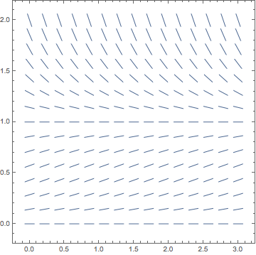
Assuming that you did the exercise correctly, you should have produced a picture that was simply a larger version of the following:

Hmmm! Here's another one where the isoclines are horizontal lines.

What about the general trend of the overall flow of the picture this time? At first glance it looks kind of like the previous example with the mirror image exponentials, but if you look very closely you will notice a few important differences:

• The horizontal slope lines are no longer in the vicinity of the x-axis, but seem to be right about the horizontal line y=1.
• The lower half of the graph isn't really exponential! The slopes are small near the x-axis, get steeper for a while, (up to about y=0.5), and then get smaller again as they approach y=1. (This is actually very hard to see with the graph Mathematica produces, and you may wish to play around with the rectangle dimensions being used in order to convince yourself of this trend.)

This kind of slope field is completely new to us! It doesn't fit into any of the categories we've seen before! We might start to wonder at this point whether it's even very important. The answer to that question is a resounding Yes!

This example is a special case of what is called the logistic model or Verhulst model for population growth. It's so important as a classic application of differential equations that we'll be doing an entire laboratory on this model later in the course.