Numerical Methods - Heun Method

Numerical Methods for Solving Differential Equations

Heun's Method

Theoretical Introduction

In the last lab you learned to use Euler's Method to generate a numerical solution to an initial value problem of the form:

y′ = f(x, y)

y(x_o) = y_o

Now it's time for a confession: In the real-world of using computers to derive numerical solutions to differential equations, no-one actually uses Euler's Method. Its shortcomings, discussed in detail in the last lab, nameley its inaccuracy and its slowness, are just too great. Though it is of some historical interest, the primary reason we bother to discuss it at all is that while it is a fairly simple algorithm to understand, it still enables us to start thinking more clearly about algorithmic approaches to the problem in general. We will now develop a better method than Euler's for numerically solving this same kind of initial value problem, but we'll use Euler's method as a foundation. For this reason Heun's Method is sometimes referred to as the Improved Euler Method.

So where should we begin? Let's start by asking what it is about Euler's Method that makes it so poor at its job. Recall that the basic idea is to use the tangent line to the actual solution curve as an estimate of the curve itself, with the thought that provided we don't project too far along the tangent line on a particular step, these two won't drift too far apart. In reality, this turns out to be asking too much. Even when extremely small step sizes are used, over a large number of steps the error starts to accumulate and the two solutions part company! We can even go so far as to theoretically predict what kind of error the method will introduce.

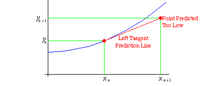
Where the actual solution curve is concave-up, its tangent line will underestimate the vertical coordinate of the next point, as seen in the image below.

Ideally, we would like our "prediction line" to hit the solution curve right at its next predicted point, as shown below.

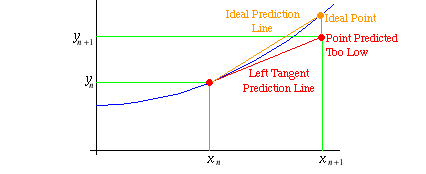
(Of course, where the actual solution curve is concave-down, the situation is reversed, and the tangent line will overestimate the vertical coordinate of the next point.)

However, we should remind ourselves that our discussion is purely theoretical. We do not really know the actual solution to the differential equation we are solving. If we did, then why would we bother trying to find a numerical solution? So in reality there is no quick way for us to know at any given stage of our numerical solution derivation whether or not the actual solution curve is concave-up or concave-down, and hence, there is no quick way to know whether or not our next calculated point is an over- or under-estimate. And remember, we don't even have any guarantee that the concavity of the curve remains consistent. It may actually change from concave-up to concave-down at some point within the domain of our desired solution.

Now let's think about how we might begin to fix this problem of the actual solution curve and the numerical solution drifting apart. Can we beat the "concavity problem?" Somehow we need to correct the over- or under-estimate problem that Euler's Method inevitably encounters. The Heun algorithm cleverly addresses this correction requirement. Let's take our concave-up example from above, and consider it more carefully this time.

Instead of focussing on the initial, left end-point where we formed our tangent line, consider the interval spanned by the tangent line segment as a whole. As we've already noted, the tangent line from the left underestimates the slope of the curve for the entire width of the interval from the current point to the next predicted point, and as a result of this, the points along the tangent line have vertical coordinates which are all underestimates of those of the points lying along the actual solution curve, including the all-important right end-point of the interval under consideration. (After all, it is this point which forms the next component of our evolving numerical solution.)

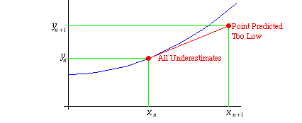
To overcome this deficiency we would need to have used a line with a greater slope in order to more accurately predict the coordinates of the next point in our numerical solution. But how much steeper should our "prediction line" be made? Some fixed percentage? Some absolute amount? Well, no, that wouldn't make sense, as differing solutions have differing curvatures, and hence would require differing correction factors. No, if we're to make our "prediction line" steeper we need to do it in some logical way which takes into account, at least to some extent, the actual shape of the solution curve.

Heun's clever approach to this problem is to consider the tangent lines to the solution curve at both ends of the interval we are investigating. As we have already established, the tangent line to the curve at the left end-point of the interval is not steep enough for accurate predictions. However if we consider the tangent line to the curve at the right end-point, (assuming we can find it somehow—more on this later,) it has the opposite problem. Look at the plot below. It shows the right hand tangent line, but since we wish to predict the next point by extrapolating from the known point we already have, i.e. the left end-point, we need to construct a prediction line based on the right tangent line's slope alone. We don't use the right tangent line itself to make our prediction, since, in a sense, it's "already there" at the right end of the interval which we are spending so much time trying to predict. So we create a line passing through our known point at the left end of the interval, and we give it the slope of the tangent line passing through the right endpoint. (You may need to read that sentence again!)

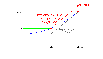
Obviously its slope is too steep to be used as the slope of our "ideal prediction line," and results in an overestimate if it is used. A few moments thought should confirm for you that this situation will always be true for any interval over which the solution curve is concave up.

Now look at the relationship between the errors made by both our left and right tangent line predictions. One is underestimating the y-coordinate of the next point, and the other is overestimating it.

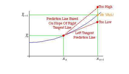
The point we really want, i.e. the "ideal point" discussed earlier, appears to lie approximately halfway between these erroneous estimates based on tangent lines. In order to get this "ideal point" we still need to ride along an "ideal prediction line," but what should we use as this line's slope? If you've really been following the foregoing discussion you can probably guess by now what slope we'll use. We will take the average of the slopes of the left and right tangent lines that we've spent so much time discussing already. (After all, a line with a slope which is the average slope of a couple of lines predicting both too high and too low respectively, should be closer to the correct value than either of them!)

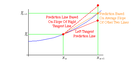
So that's the basic idea behind Heun's method—using a prediction line whose slope is the average of the slopes of the tangent lines at either end of the interval.

Now we have to tackle a problem that I hinted at earlier: We don't actually know the right end-point of the interval, and therefore there is no way to know the slope of the tangent line at that point! (If we did know the right end-point's coordinates then we wouldn't be wasting our time trying to find them with this algorithm!) Recall that in the last lab we learned how to use Euler's method to find the approximate location of the next point along a solution curve? That's what we'll do with Heun's method! We'll use Euler's method to roughly estimate the coordinates of the next point in the solution, and once we have this information, we'll re-predict (or correct) our original estimate of the location of the next solution point by using the method of averaging the slopes of the left and right tangent lines that we so carefully developed above.

(As a side note, numerical analysts would refer to Euler's method as a predictor algorithm, whereas Heun's method is described as a predictor-corrector algorithm. Can you see why they would use this kind of nomenclature?)

OK, since we've managed to conceptualize the Heun algorithm graphically, it's now time to develop the method symbolically so that we can more easily see how to write the Mathematica code for it.

We already have our iterative formulas from the previous lab on Euler's method to get the ball rolling. These were:

x_n+1 = x_n +  h

y_n+1 = y_n +  h f(x_n, y_n)

where f(x, y) was the right-hand side of the original differential equation, and h is the width of the subdivisions we are planning to use. Also, (x_n, y_n) represented the known (left) point, and (x_n+1, y_n+1) represented the new (right) point. Remember, the reason we care about these formulas for our new Heun method is that we'll be using Euler's method to make a rough prediction of the location of the predicted next point so that these coordinates may be used for our estimate of the slope of the tangent line at the right end of the interval in question.

So let's get those tangent line slopes figured out formulaically.

The left end-point is simply the current point, (x_n, y_n), so the slope of the tangent line at the left end-point, just as with Euler's method, is the right hand side of the original differential equation evaluated at this point:

slope_left = f(x_n, y_n)

Now for that right end-point that we've been worrying about so much. As we said just a few seconds ago, Euler gives a rough prediction of its location as being at coordinates:

(x_n+1, y_n+1) = (x_n + h, y_n +  h f(x_n, y_n))

Recalling that one of our fundamental assumptions, based on our interpretation of the original differential equation, is that the quantity f(x, y) on the right hand side of the equation can be thought of as the slope of the solution we seek at any point (x, y), we may now combine this idea with the rough, Euler estimate of the next point to give us an estimate of the slope of the tangent line at the right end-point. This would be:

slope_right = f(x_n + h, y_n +  h f(x_n, y_n))

Next, recall from the discussion and the graphs we considered above that the slope of our "ideal prediction line" is the average of the left and right tangent slopes whose formulas we have just found. In other words:

slope_ideal = (1/2) (slope_left + slope_right)

All that is left to do now is to utilize this slope in creating the "ideal prediction line" itself, and then use this "ideal prediction line" to actually find the coordinates of the right hand end-point. To a great extent the remainder of the work is simply a repetition of what we saw as we developed the formulas for Euler's method in the last lab.

Consider the following illustration. We wish to predict the right hand end-point's coordinates. In order to get them it would be sufficient to find the value of Δy.

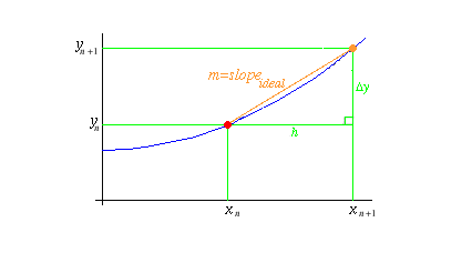
Using the elementary idea that slope = rise / run, we derive the following formula immediately from the picture:

slope_ideal =  Δy / h

which is easily rearranged to give us a formula for Δy, namely:

Δy = h slope_ideal

Finally, then, we can predict the coordinates of the next point in our numerical solution. The next x-coordinate is simply the current x-coordinate plus the step size, h. The next y-coordinate is the current y-coordinate plus Δy. Formulaically, this would be:

x_n+1 = x_n + h

and

y_n+1 = y_n + Δy

Replacing Δy by the value we just found for it above, this becomes:

y_n+1 = y_n + h slope_ideal

And replacing slope_ideal by the average of the left and right tangent slopes found earlier, this is transformed into:

y_n+1 = y_n + (1/2) h (slope_left + slope_right)

One last substitution, and our formula is complete. We recently found that:

slope_left = f(x_n, y_n)

and that

slope_right = f(x_n + h, y_n +  h f(x_n, y_n))

so if we substitute these values into the above equation for y_n+1 we get:

y_n+1 = y_n + (1/2) h (f(x_n, y_n) + f(x_n + h, y_n +  h f(x_n, y_n)))

or, cleaning things up slightly:

y_n+1 = y_n + (h/2) (f(x_n, y_n) + f(x_n + h, y_n +  h f(x_n, y_n)))

At last! We're done with our theory for Heun's method. Summarizing the results, the iteration formulas for Heun's method are:

x_n+1 = x_n + h

y_n+1 = y_n + (h/2) (f(x_n, y_n) + f(x_n + h, y_n +  h f(x_n, y_n)))

It's now time to implement these newly minted formulas in Mathematica.

---

If you're lost, impatient, want an overview of this laboratory assignment, or maybe even all three, you can click on the compass button on the left to go to the table of contents for this laboratory assignment.